MIKE SHE Python API

This section describes the MShePy module, which enables the use of Python scripting with MIKE SHE. This includes:

1. running Python plugins during a MIKE SHE simulation;

2. running MIKE SHE simulations from Python scripts.

In the first case, the user can add plugins to a MIKE SHE model. A plugin consists of a collection of code functions in Python performing custom func­tionalities. During preprocessing, the Python plugins are attached to the model and once the simulation is started, functions (or "slots") in the plugins will be connected to signals that MIKE SHE will emit during the simulation, e.g. after initialization or before a time step. Once the function has finished to perform arbitrary tasks (e.g. exchange data with MIKE SHE), MIKE SHE will continue the normal execu­tion.

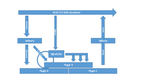
In the second case, the user can call and execute the water movement engine of a MIKE SHE model from a Python shell. This allows controlling the simulation time from the Python shell and exchange items between the MIKE SHE model and the Python environment before, during, and after the simulation.

Requirements

The MShePy module is available from MIKE Zero 2019 version 1. Only water movement (WM) can be accessed through MShePy. Thus, water quality sim­ulations, the preprocessor and other components are currently not supported.

All water movement components can be accessed by MShePy. This includes:

• Overland flow
• River exchange items
• Unsaturated flow
• Evapotranspiration
• Saturated flow

Python versions supported by MIKE SHE:

MIKE SHE versions	Supported Python Versions (64 bit only)
2021.1, 2022	3.7, 3.8, 3.9
2021	3.7, 3.8
2020.1	3.6, 3.7, 3.8
2019.1, 2020	3.6, 3.7

Python is not included with the MIKE SHE installation, it can be download from various places, e. g. https://www.python.org/.

Python Plugins

How to enable Python plugins in the MIKE SHE user interface

In the Simulation Specification panel (below), tick the Enable Plugins option.

Then open the Python Plugins panel. Under Python Library you can specify how to find the Python dynamic library. "Search default locations" means the operating system´s default search order will be used. On MS Windows this is the application´s directory, several system folders, the current directory and directories in the system PATH variable. The most recent Python version will be preferred. When you tick "Specify" instead you can provide the location of the Python library file (e.g. python38.dll for version 3.8 and python39.dll for version 3.9).

Use the insert button to add plugin files to the simulation. Several plugin files can be added to the same MIKE SHE model. Provide the location of the plugin Python file (*.py) and tick the box in the "Enable"-column to activate a plugin file. The order of plugin files in this table will determine the order of execution during the simulation.

Creating a Python plugin

The first step is to import the MShePy module by the command import MShePy. The command will import the MShePy version corresponding to the specified Python library version (see previous section).

The second step is to define at which point of the simulation custom functions defined in the plugin should be executed. MIKE SHE emits six different sig­nals at predefined moments in the simulation. For each signal that is being emitted, one or more plugin functions can be executed. The connection between the signal and the plugin function (or "slot") is simply made by a naming convention. The function definitions are shown in the Table below.

Function definitions

Moment in the simulation	Python function definition
During early initialization	def enterSimulator():
At the end of the initialization	def postEnterSimulator():
At the beginning of each time step	def preTimeStep():
At the end of each time step	def postTimeStep():
After the last time step	def preLeaveSimulator():
Right before closing MIKE SHE, after output files (including logfiles!) have been closed	def leaveSimulator():

The third step is to describe actions, which are executed at the defined moments during the simulation, possibly using functions available in the Python environment. An overview of functions included in the MShePy library is provided in the following section. The same plugin file can contain different functions executed at different moments in the simulation. A simple example is shown below for a function printing in the log file the initial timestep count (0) and then the timestep number at each timestep:

import MShePy # Import MShePy module  

timestep = 0 # Define a global variable

def enterSimulator(): # Define the slot/function
   global timeStep
   MShePy.wm.log("The timestep is {0}".format(timeStep)) # Print initial timestep in log file  

def postTimeStep(): # Define the slot/function
   global timeStep
   MShePy.wm.log("The timestep is {0}".format(timeStep)) # Print timestep in log file
   timeStep += 1 # Calculate next time step

Functions available in the MShePy library

The MShePy library provides functions to exchange items between the Python script and the MIKE SHE simulation. An overview of the functions exposed by the MShePy library is given in the table below. All functions can be called by typing MShePy.wm.* followed by the name of the function (e.g. (MShePy.wm.getValues).

Help for the MShePy module can be obtained by typing help(MShePy) in a Python terminal, a description of a specific function can be obtained by typing e. g. help(getValues).

Functions available in the MShePy library

Function	Description	Parameters	Return value
getValues(paramTypeId)	Get a copy of values of a MIKE SHE item from a current simula­tion	paramTypeId is the Id of the MIKE SHE parameter to get	A tuple: Initial time step (datetime.date­time object), current time step(date­time.datetime object), dataset object
setValues(dataset)	Set values to the cur­rent MIKE SHE simu­lation	Dataset object	None
gridGeoInfo()	Get the model projection, grid origin and rotation. The origin is the center of the lower left cell of the model domain.	None	Tuple: projection (string), x-origin (double), y-origin (double), rotation (double)
gridCellToCoord(ix, iy)	From x, y cell index get the coordinates in the models coordi­nate system	ix (int): cell x-index; iy (int): cell y-index	cell coordinate in x-direction, cell coordi­nate in y-direction
gridCoordToCell(dx, dy)	From x, y coordinates in the models coordi­nate system get the x, y cell index	dx (double): cell x-coordinate; dy (double): cell y-coordinate	cell index in x-direc­tion, cell index in y-direction
gridIsInModel(ix, iy)	Is this cell (2d cell indi­ces) inside the model area (internal or boundaries)?	ix (int): cell x-index; iy (int): cell y-index	True or False
gridIsInternal(ix, iy)	Is this cell (2d cell indi­ces) inside the model area (excluding boundaries)?	ix (int): cell x-index; iy (int): cell y-index	True or False
log(*args)	Send a message to the MIKe SHE log file	arbitrary num­ber of objects.	None
print(*args)	Send a message to the MIKE SHE print-log file, in the result folder	args: arbitrary num­ber of objects.	None
currentTime()	Get the current time step	None	Datetime.datetime object
nextTimeStep()	Get the length of next unsaturated zone (UZ) and saturated time (SZ) steps	None	length of next UZ time step in hours, length of next SZ time step in hours
simPeriod()	Get the start and end date time for the cur­rent simulation.	None	Initial time step (date­time.datetime object) and end time step (datetime.datetime object)

How to exchange MIKE SHE items with Python

MShePy provides access to certain MIKE SHE exchange items. Some of these are both for in- and output, others for either in- or output only. All MIKE SHE items that can be accessed from Python are listed in the sum­mary tables at the end of this chapter. The availability of MIKE SHE items depends on the components selected in the "Simulation specification" panel. For example, if the evapotranspiration component is not included in the simula­tion, then no parameters related to evapotranspiration will be available. The accessible variables are listed in the _WM.log file, once preprocessing and water movement initialization has been executed. Some items will only be available when the extra parameter "expose da items" is specified and set to true*.

In order to exchange MIKE SHE items between the Python plugin and the MIKE SHE simulation two functions are available in the MShePy module:

• MShePy.wm.getValues() to retrieve a copy of items from MIKE SHE to Python;
• MShePy.wm.setValues() to change the value of MIKE SHE items in the simulation.

The input of the MShePy.wm.getValues() is a MIKE SHE parameter ID. The predefined parameter IDs are available from MShePy.paramTypes.* followed by the abbreviation corresponding to the parameter (see summary tables at the end of this chap­ter for the list of abbreviations). The output of the getValues function is a tuple containing the starting time as a datetime.datetime object, the current time as another datetime.datetime object, and a MshePy dataset containing the value of the selected MIKE SHE item (see following section for a description of the M­ShePy dataset type). For example you could do this:

>>> (dtStart, dtEnd, values) = MShePy.wm.getValues(MShePy.paramTypes.P_RATE)
>>> dtStart
(datetime.datetime(2000, 1, 5, 22, 0),
>>> dtEnd
datetime.datetime(2000, 1, 6, 0, 0),
>>> values
MShePy36.dataset: "precipitation rate", Precipitation Rate (meter/sec), in: Global value, out: BaseGrid, shape: [100, 3], size: 296)

The input to MShePy.wm.setValues() is a MShePy dataset.

How to create and handle MShePy datasets

The function MShePy.dataset() can be used to create a dataset. The argu­ment of the function is a MIKE SHE parameter ID (MShePy.paramTypes.*). The characteristics of the dataset, such as the dimension and the unit, depend on the properties of the selected MIKE SHE parameter and will be automatically set to match the current model setup. So before calling this function the initialization of the model must have been completed. An overview of the available parameters, their properties and corresponding IDs is given in the summary tables at the end of this chapter.

The string representation of a MShePy dataset object contains some of its properties (see example below). The displayed properties include:

• The parameter description (e. g. "precipitation rate")
• The current unit (e. g. meter/sec)
• The input and output dimension (e. g. "Global value")
• The shape (number of elements in each dimension)
• The size, or total number of elements inside the model area. Note that this number is usually lower than the product of the extents in each dimension, as most models are not box-shaped – cells outside the model boundary, but inside the model domain bounding box will not be counted.

MShePy dataset objects can be indexed using square brackets. The number of inputs in the square brackets depends on the dimension of the object. For instance, 2 inputs can be given for the precipitation rate object in the example below (e. g. data[1,1]). Slices can be selected by using the colon (e. g. data[1:3,1], data[:,1] or data[1:3:2,1]). The *.value() attribute can also be used to display all values inside a MShePy dataset, or to change all values in a dataset by specifying the new value as an argument (e. g. data.value(10.0)):

>>> (startTime, endTime, data) = MShePy.wm.getValues(MShePy.param­Types.P_RATE)
>>> data
MShePy36.dataset: "precipitation rate", Precipitation Rate (meter/sec), in: Global value, out: BaseGrid, shape: [100, 3], size: 296
>>> data[1,1]
0.0
>>> data[1:3,1]
[0.0, 0.0]
>>> data.value(10.0)
>>> data[1:3,1]
[10.0, 10.0]

The dimension shown in the summary tables at the end of this chapter refers to the standard dimension the MIKE SHE item has, which is also the dimen­sion the output item has. However, the real dimension of input items may be different, depending on the selected option in the MIKE SHE interface. For example, the precipitation rate is usually 2 dimensional (BaseGrid in the previous example), but the input item can also be a global value when the option Uniform is selected in the Precipitation Rate dialog in the MIKE SHE user interface (see figure below).

The number of elements in each dimension of a MShePy dataset object can be retrieved by the function shape(). In the example below, data.shape() returns [100,3]. Similarly, size() function returns the total number of ele­ments in a MShePy dataset object (e.g. 196), or the extent in a given dimen­sion when the index of the dimension is given as a parameter, e.g. size(1).

In order to retrieve the unit of a MShePy dataset object, the function unit() is available. No arguments are required and the function returns the unit of the dataset object. Note that this unit may be different from the unit selected in the MIKE SHE GUI. In the following example, data.unit() would return 'meter/sec', while the default unit of the precipitation rate in the MIKE SHE GUI is 'mm/d'.

>>> data
MShePy36.dataset: "precipitation rate", Precipitation Rate (meter/sec), in: Global value, out: BaseGrid, shape: [100, 3], size: 296
>>> data.shape()
[100, 3]
>>> data.size()
296
>>> data.unit()
'meter/sec'

In the Python environment, the unit of a MShePy dataset object can be changed by using the function convert(). The argument to the function is the new unit as text (e. g. value.convert('mm/year')). Each MShePy dataset can be con­verted to a unit matching the corresponding item type. The valid units for a given item type can be found in the GUI under File->Options->Edit Unit Base Groups. The unit conversion in Python will not affect the units of the regular MIKE SHE grid- or detailed time series output items. It is not required to reset the unit before committing the dataset with the setData method: This will be taken care of by the MShePy module.

It is also possible to set a different unit without doing any conversion by call­ing unit() with an argument. This may be useful when creating a new data­set or for setting the correct unit when making calculations that are supposed to result in a different unit.

>>> (startTime, endTime, data) = MShePy.wm.getValues(MShePy.para­mTypes.SZ_HEAD)
>>> data[20,22,1]
9.202210426330566
>>> data.unit() # get default unit
'meter'
>>> data.convert("inch") # invalid conversion, see error message:
Traceback (most recent call last):   File "<stdin>", line 1, in <module>
LookupError: "inch" is a known unit, but it does not match the item type "Elevation" of the dataset.
>>> data.convert("feet")
MShePy36d.dataset: "head elevation in saturated zone", Elevation (feet), in: SZ3DGrid, out: SZ3DGrid, shape: [50, 50, 3], size: 5652
>>> data[20,22,1] # get the value that now is in feet (compare to above data[...] statement!)
30.190979089011048

The MShePy library allows arithmetic operations with MShePy datasets: addition, subtraction, multiplication, division, exponentiation, absolute value, negative value, and positive value using standard Python syntax. The resulting MShePy dataset will have the properties of the first MShePy dataset in the equation (in the example below, NEW is the same dataset type as HEAD, while NEW1 is the same as ET).

Arithmetical operations where MShePy datasets are sliced using square brackets( e.g. ET[:] = HEAD[:,:,0]), will not replace the dataset object, but only the values inside it.

>>> (startTime, currentTime, ET) = MShePy.wm.getValues(MShePy.par­amTypes.ET_REF_EXC)
>>> (startTime, currentTime, HEAD) = MShePy.wm.getVal­ues(MShePy.paramTypes.SZ_HEAD)

>>> NEW = HEAD + ET
>>> NEW
MShePy36.dataset: "head elevation in saturated zone", Elevation (meter), out: SZ3DGrid, shape: [100, 3, 1], size: 296

>>> NEW1 = ET + HEAD
>>> NEW1
MShePy36.dataset: "reference evapotranspiration (OpenMI)", Evapo­transpiration Rate (meter/sec), in: Global value, out: BaseGrid, shape: [100, 3], size: 296

>>> ET[:] = HEAD[:,:,0]
>>> ET
MShePy36.dataset: "reference evapotranspiration (OpenMI)", Evapo­transpiration Rate (meter/sec), in: Global value, out: BaseGrid, shape: [100, 3], size: 296

Running MIKE SHE simulations from Python scripts

This section describes the steps to execute a MIKE SHE model using a Python script. Functions are included in the MShePy module to initiate and run a MIKE SHE simulation from a Python script.

The MIKE SHE model has to be preprocessed before it can run using the MShePy module. The MIKE SHE model can contain Python plugins.

Limitations

Each python process can be used for the execution of just one single MIKE SHE model. It is not possible to

• run more than one model in parallel in the same process or
• run more than one model sequentially.

If it is required to run several MIKE SHE models sequentially or in parallel this can be achieved by invoking an additional python process for each model and starting MIKE SHE in that sub-process.

Initializing a MIKE SHE model

The MShePy module resides in the MIKE installation´s bin/x64 folder. This needs to be in your search path for python modules, e.g. by calling sys.path.append([MIKE installation]/bin/x64). Import the MShePy module by using the command import MShePy.

In order to initialize the MIKE SHE model, use the MShePy.wm.initial­ize(r"*.she") function. The function argument is the path to the MIKE SHE model file. While a MIKE SHE model is initialized from a Python script, the model can be opened, but not run in MIKE ZERO.

Running MIKE SHE water movement

Three functions are available in the MShePy module to perform one or more timesteps in the MIKE SHE model:

• MShePy.wm.runAll() which performs the entire simulation. When using this method you must not initialize or terminate the simulation, differently from the other functions;
• MShePy.wm.performTimeStep() which performs one timestep
• MShePy.wm.runToTime(time) which performs timesteps until reaching the specified time (a datetime.datetime object). WARNING: Be aware that sources and sinks assigned from the Python script (including parameters such as a fixed hydraulic head which are con­verted to sources/sinks in the MIKE SHE engine) will remain active for all time steps taken during the execution of this method and be reset only right before the method returns.

All MShePy functions can be called to retrieve and assign variable values in MIKE SHE during the simulation.

Termination and postprocessing

The function MShePy.wm.terminate(success) can be used to terminate the simula­tion. The user should provide as function input False if an error occurred dur­ing the simulation or True if no error occurred.

Postprocessing and the visualization of the results can be done in MIKE ZERO and MIKE VIEW. Results can also be exported using Python and han­dled in an external software. Further processing could also be done in Python, e. g. using the MIKE SDK via the PythonNet package. See the MIKE SDK documentation for further details.

Python script example

A simple Python script initializing, running and terminating a MIKE SHE model is shown below:

import datetime                                    # Import datetime module
import MShePy                                      # Import MShePy module
MShePy.wm.initialize(r"C:\Users\PETR.she")         # Initialize the model
currentTime = MShePy.wm.currentTime()              # Find the initial timestep
EndTime = currentTime + datetime.timedelta(days=5) # Calculate the end timestep after 5 days
MShePy.wm.runToTime(EndTime)                       # Run the model until the specified timestep
MShePy.wm.terminate(True)                          # Terminate the simulation
# (guards against executing a script on import omitted!)

Plugins application example

Calculation of reference evapotranspiration

Several methods are available to calculate the reference crop evapotranspi­ration, depending on the data available. One of these methods is the Blaney-Criddle equation from Brouwer and Heibloem (1986):

where ET_0 is the reference evapotranspiration as an average of a period of one month [mm/day], p is the mean daily percentage of annual daytimehours, and Tmean is the daily mean air temperature [C].

The following Python plugin calculates the reference evapotranspiration for a 1-year MIKE SHE simulation using the Blaney-Criddle method according to the example provided by Brouwer and Heibloem (1986).

The plugin is composed of three parts: 1. Importing MShePy module 2. Creating global variables (P, T_max, and T_min) 3. Calculating and assigning the evapotranspiration at the beginning of each time step.

In order to calculate the evapotranspiration (point 3), an MShePy.dataset object containing evapotranspiration values is created. Since the temperature and the percentage of daytime hours is given in monthly average, the month of the current time step is used to select the corresponding values for the month. These values are used to cal­culate the reference evapotranspiration value and assign it to the MIKE SHE simulation. For this example, the evapotranspiration value was chosen to be a global value for the whole model domain.

import MShePy # import the MShePy module

# define global variables
# monthly average of percentage of daytime hours
P     = [0.26, 0.26, 0.27, 0.28, 0.29, 0.29, 0.29, 0.28, 0.28, 0.27, 0.26, 0.25]
# monthly average of daily maximum temperature (℃)
T_max = [32.1, 35.8, 38, 38.7, 39, 36.6, 32.6, 30.8, 31.8, 34.8, 35, 32]     
# monthly average of daily minimum temperature (℃)
T_min = [15.5, 18.8, 21.8, 24.5, 26, 25, 22.7, 22, 23, 21.3, 18.7, 16.6]     

def preTimeStep():                                      # define the preTimeStep slot
  PET    = MShePy.dataset(MShePy.paramTypes.ET_REF_EXC) # Create PET dataset
  time   = MShePy.wm.currentTime()                      # Find current time step
  month  = time.month                                   # Find current month
  T_mean = (T_max[month-1] + T_min[month-1]) / 2        # Average temperature
  ET     = P[month-1] * (0.46 * T_mean + 8)             # Calculate ET (mm/d)
  PET.value(ET)                                         # Assign value to PET dataset
  MShePy.wm.setValues(PET)                              # Assign ET value to simulation

Reference evapotranspiration adjusted for altitude

Reference evapotranspiration can be calculated using the modified ver­sion of the Penman-Monteith equation presented by Allen et al. (1998):

where ET_0 is the refence evapotranspiration [mm/day], R_n is the net radiation at the crop surface [MJ/m2/day], G is the soil heat flux density [MJ/m2/day], T is the mean daily air temperature at a 2 m height [oC], u2 is the wind speed at a 2 m height [m/s], e_s is the saturation vapor pressure [kPa], e_a is the actual vapor pressure [kPa], D is the slope vapor pressure curve [kPa/oC], and g is the psychrometric constant [kPa/oC].

This plugin example considers the changes in pressure and, thus, on the psy­chrometric constant due to the elevation. The psychrometric constant can be expressed as function of the elevation:

where Z is the ground elevation [m].

The plugin below reproduces example 17 by Allen et al. (1998). It consists of three parts:

• Importing MShePy module
• Creating global variables
• Calculating and assigning the evapotranspiration at the end of the initial­ization

The calculation of the g and, thus, of the evapotranspiration depends on the surface elevation. In the plugin example, Gamma (g) is calculated using Ele­vation, which is a MShePy dataset for surface elevation. Thus, Gamma is also a MShePy surface elevation dataset, but it contains value of g, whose unit is [kPa/oC] and not [m]. This is also true for the ET variable, which con­tains the calculated evapotranspiration. This discrepancy is solved by assign­ing the value of ET to PET, which is a MShePy reference evapotranspiration dataset. It would not be possible to calculate the values of PET directly from an elevation dataset, because the elevation dataset cannot be changed to a PET dataset.

import MShePy # import the MShePy module

# global variables
Delta = 0.246 # Slope vapour pressure curve (oC/kPa)
Rn    = 14.33 # Net radiation at the crop surface (MJ/m2/day)
G     = 0.14  # Soil heat flux density (MJ/m2/day)
T     = 30.2  # Monthly average mean temperature (oC)
u2    = 2     # Monthly average daily wind speed measured at 2 m (m/s)
Es    = 4.42  # Monthly average daily saturation vapour pressure (kPa)
Ea    = 2.85  # Monthly average daily actual vapour pressure (kPa)

def postEnterSimulator(): # define the slot
  # Create PET dataset
  (startTime, currentTime, PET) = MShePy.wm.getValues(MShePy.param­Types.ET_REF_EXC)
  PET.convert('mm/day')                  # Convert the unit of the PET dataset

  # Get the elevation from the MIKE SHE model
  (startTime, currentTime, Elevation) = MShePy.wm.getVal­ues(MShePy.paramTypes.DEM_Z)

  # Calculate the psychrometric constant from the elevation (kPa/oC)
  Gamma = 0.00065 * 101.3 * ((293 - 0.0065 * Elevation) / 293)**5.26

  # Calculate reference ET (mm/d)
  ET = (0.408 * Delta * (Rn - G) + Gamma * (900 / (T + 273)) * u2 * (Es - Ea)) / (Delta + Gamma * (1 + 0.34 * u2))
  PET[:] = ET[:]           # Assign calculated value to PET dataset
  MShePy.wm.setValues(PET) # Assign evapotranspiration value to the simulation

Managing irrigation as a function of precipitation in the previous months

Periods with dry conditions will typically require more irrigation compared to wet periods. The following plugin implements a simplified method to optimize the irrigation rate based on the precipitation rate of the previous weeks.

At the beginning of each time step, the precipitation rate of the previous month, compared to the current simulation time step, is analyzed. For precip­itation rates lower than the annual mean precipitation rate, irrigation is applied to the model. When the previous month has been a wet one (precipitation rate higher than the annual mean), then no irrigation is applied.

In this plugin, the irrigation rate is applied to the model as part of the precipita­tion rate. Thus, a new precipitation rate is calculated as the sum of the observed precipitation and calculated irrigation and passed to the MIKE SHE simulation. For simplicity it is assumed that the water originates from outside the model. If required the water could however also be taken from inside the model, e. g. by extracting water from the saturated zone. It is then the users responsibility to maintain the water balance. Any effective water balance error would not be flagged as an error in the MIKE SHE water balance provided my MIKE SHE, as the source (irrigation) and the sink (e. g. SZ extraction) are not being matched – MIKE SHE will treat both sink and source as if they were independantly removing/adding water out of/into the model.

import MShePy

Precipitation = [1.3, 0.7, 1.3, 1, 1.3, 2, 1.9, 1.9, 2, 1.6, 2, 1.6] # Monthly average precipitation (mm/d)

P_mean = 1.6 # Annual mean precipitation (mm/d)

def preTimeStep():
  PreIrr = MShePy.dataset(MShePy.paramTypes.P_RATE) # Cre­ate Precipitation+irrigation dataset
  time = MShePy.wm.currentTime()                    # Current time step
  month = time.month                                # Current month in the simulation
  if Precipitation[month-2] < P_mean:   # Condition for irrigation
    Irrigation = P_mean - Precipitation[month-2]      # Calculate the irri­gation rate (mm/d)
    PreIrr_rate = Precipitation[month-1] + Irrigation # Calculate irriga­tion + recharge (mm/d)
    PreIrr.value(PreIrr_rate)                         # Assign irrigation + recharge
  else:
    PreIrr.value(PreIrr_rate)                       # Assign recharge rate

  MShePy.wm.setValues(PreIrr) # Commit values

Summary tables of exchange items between MIKE SHE and Python

Overview of MIKE SHE items that can be exchanged as input with Python. The dimension may change for input items depending on the selected option for the item in the MIKE SHE interface. The unit may also change depending on the option selected in File->Options->Edit Unit Base Groups.

Input items

Parameter	Abbreviation	Unit	Dimension
Precipitation rate	P_RATE	m/s	2
Air temperature	AIR_TEMP	C	2
Rooting depth	ROOTZONE_WC	m	2
Leaf area index	LAI		2
Crop coefficient	KC		2
reference evapotranspiration	ET_REF_EXC	m/s	2
updated precipitation rate	P_RATE_UPDT	m/s	2
depth of overland water	OL_D	m	2
External sources to Overland (for OpenMI)	OL_SOURCE	m3/s	2
overland water elevation	OL_H	m	2
Inflow (flux) to OL drain	OLDR_IN_FLX	m/s	2
Inflow (flow) to OL drain	OLDR_IN_FLO	m3/s	2
water content in unsaturated zone	UZ_WC		3
SZ head elevation of layer	SZ_HEAD_LY	m	2
head elevation in saturated zone	SZ_HEAD	m	3
SZ horizontal conductivity (for DA-OpenMI)	SZ_K_HOR	m/s	3
SZ vertical conductivity (for DA-OpenMI)	SZ_K_VER	m/s	3
Leakage (flux) to SZ	SZ_LEAD_FLX	m/s	2
Leakage (flow) to SZ	SZ_LEAK_FLO	m3/s	2
Inflow (flux) to SZ drain	SZDR_IN_FLX	m/s	2
Inflow (flow) to SZ drain	SZDR_IN_FLO	m3/s	2
External sources to SZ layer	SZ_SOURCE_LY	m3/s	2
groundwater extraction	SZ_EXTR	m3/s	3
External sources to SZ (for OpenMI)	SZ_SOURCE	m3s	3
pumping from baseflow reservoir	PMP_BASE	m3/s

This table is an overview of MIKE SHE items that can be exchanged as out­put with Python. The dimension may change for input items depending on the selected option for the item in the MIKE SHE interface. The unit may also change depending on the option selected in File->Options->Edit Unit Base Groups.

Output items

Parameter	Abbreviation	Unit	Dimension
precipitation rate	P_RATE	m/s	2
air temperature	AIR_TEMP	C	2
average water content in the rootzone	ROOT_DPTH		2
rooting depth	ROOTZONE_WC	m	2
leaf area index	LAI		2
crop coefficient	KC		2
reference evapotranspiration	ET_REF_EXC	m/s	2
precipitation rate of next time step	P_RATE_NEXT	m/s	2
updated precipitation rate	P_RATE_UPDT	m/s	2
ETref x Kc	ET_REF_X_KC	m/s	2
actual evapotranspiration	ET_ACT	m/s	2
actual transpiration	TRANSP_ACT	m/s	2
actual soil evaporation	ESOIL_ACT	m/s	2
actual evaporation from interception	EI_ACT	m/s	2
actual evaporation from ponded water	EOL_ACT	m/s	2
canopy interception storage	SI	mm	2
evapotranspiration from SZ	ESZ	m/s	2
snow evaporation	SNOW_ET	m/s	2
depth of overland water	OL_D	m	2
overland flow in x-direction	OL_FLOW_X	m3/s	2
overland flow in y-direction	OL_FLOW_Y	m3/s	2
OL Drain Storage Depth	OLDR_S	m	2
net precipitation rate for AD	P_NET_AD	m/s	2
overland water elevation	OL_H	m	2
net input to overland (flux)	OL_IN_NET_FLX	m/s	2
net input to overland (flow)	OL_IN_NET_FLO	m3/s	2
infiltration to UZ (negative)	INF	m/s	2
exchange between UZ and SZ (pos.up)	UZ_SZ_EX_POSUP	m/s	2
bypass flow UZ (negative)"	BYP_FLO	m/s	2
total recharge to SZ (pos.down)	RECHARGE_POSDN	m/s	2
total recharge (flow) to SZ (pos.down)	RECH_TOT_FLO	m3/s	2
groundwater levels used by UZ	GW_LVL	m	2
unsaturated zone flow	UZ_FLO	mm/h	3
water content in unsaturated zone	UZ_WC		3
root water uptake	ROOT_UPTK	m/s	3
macropore water content	MP_WC		3
macropore flow	MP_FLO	mm/h	3
exchange from matrix to macropores	MX_MP_EX	mm/h	3
exchange from macropores to matrix	MP_MP_EX	mm/h	3
depth to phreatic surface (negative)	PHR_DP	m	2
elevation of phreatic surface	PHR_ELV	m	2
SZ head elevation of layer	SZ_HEAD_LY	m	2
head elevation in saturated zone	SZ_HEAD	m	3
SZ horizontal conductivity (for DA-OpenMI)	SZ_K_HOR	m/s	3
SZ vertical conductivity (for DA-OpenMI)	SZ_K_VER	m/s	3
seepage flow SZ -overland	SZ_OL_EX	mm/day	2
seepage flow overland - SZ (negative)	OL_SZ_EX	mm/day	2
SZ baseflow to river of layer	SZ_RI_EX_FLO	m3/s	2
SZ drainage flow of layer	SZDR_LY_FLO	m3/s	2
SZ flow to MOUSE of layer	SZDR_MOUSE_FLOW	m3/s	2
3D UZ recharge to SZ (negative)	SZ_RE_NEG	mm/day	3
groundwater flux in x-direction	SZ_X_FLO	m3/s	3
groundwater flux in y-direction	SZ_Y_FLO	m3/s	3
groundwater flux in z-direction	SZ_Z_FLO	mm/day	3
groundwater extraction	SZ_EXTR	m3/s	3
SZ exchange flow with river	SZ_RI_EX	m3/s	3
SZ drainage flow from point	SZDR_POINT_FLO	m3/s	3
SZ flow to MOUSE	SZ_MOUSE_FLO	m3/s	3
pumping from baseflow reservoir	PMP_BASE	m3/s
overland to river flow (positive)	OL_RI_POS	m3/s
river to overland flow (negative)	RI_OL_NEG	m3/s
positive baseflow (SZ to river)	SZ_RI_POS	m3/s
negative baseflow (river to SZ)	RI_SZ_NEG	m3/s
exchange from mike 11 river to SZ	RI_SZ_EX	m3/s
exchange from mike 11 river to OL	RI_OL_EX	m3/s
river water level	RI_WL	m	2
elevation of ground surface	DEM_Z	m	2