DFS File System

Introduction

The DFS (Data File System) is used extensively within the MIKE Powered by DHI software.

It is a binary data file format and it provides a general file format for handling spatially distributed and time dependent data, ranging from measurements of temperature at a single point, Figure 1.1, to water levels in the North Sea in a 2D grid generated by DHI’s flow models (MIKE 21), Figure 1.2.

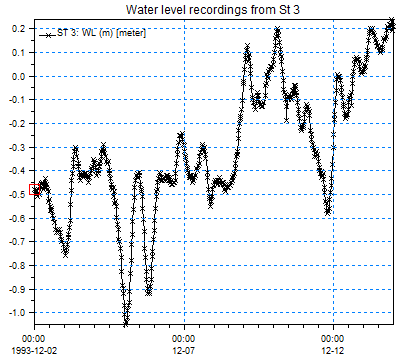
Figure 1.1 Example from dfs0 file, water level measurements from Station 3

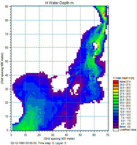
Figure 1.2 Example from dfs2 file, first time step of a 2D water level item

DFS File Contents

A DFS file is a binary file that contains data for a number of quantities at a number of times.

A DFS file is conceptually split into:

• A header section, containing general information for the file, as start time, geographic map projection, etc.

• A section with static data, containing data for a number of items. Static data does not have any notion of time, and is thus independent of time.

• A section with dynamic data, containing data for a number of time steps and items.

Figure 2.2 DFS file contents

The Dynamic data section is usually by far the section using most disc space.

Header

The header contains metadata describing the file, its contents and especially the contents of the two data sections.

• File title; user defined title of the file.

• Application title; title of the application that created the file.

• Application version number; version of the application that created the file.

• Data type; used to tag the file as a special DFS file type, see (1) below.

• Type of DFS file storing format, see (2) below.

• Type of statistics; the level of statistics stored for dynamic items.

• Delete values, see (3) below.

• Geographic map projection information.

• Time axis information.

• Custom blocks; a number of (small) arrays of a certain type, identified by its name.

• Compression encoding; when the file is compressed, defines where compressed data point belongs to.

Furthermore, the header contains descriptions of each of the dynamic items. The header does not contain any information on the static items; neither does it contain the number of static items in the file. Static items must be read one by one until there is no more. A read operation will provide as well static item data as information on the static item.

The type of statistics, geographic map projection information, time axis information, custom blocks and compression encoding is described in the next sections.

1. The data type tag is a user specified integer. The data type tag is used as an identification tag for the type of DFS file at hand. The user should tag bathymetries, result files, input files etc. matching those tags required for the DFS file type at hand. A wrong data type tag in some contexts is an error. Not all DFS files and tools handling DFS use the tag.

   In Appendix G there is a list of data type tags currently used within the DHI model complex. A programmer writing a new type of DFS file should choose the tag carefully, such that it does not interfere with existing DFS file types.

2. The storing format specifies whether all items are stored in all time steps, and if a time-varying spatial axes is used. Currently the DFS file system only supports files with all items in all time steps and not any of the time-varying spatial axes. Thus this is not used, and is not presently planned to be explored.

3. A delete value represents a not-defined value. If a value is not available, or if it does not make sense to set a value, setting the delete value indicates that there is no value. There is a delete value for data of type float, double, integer (32 bit), unsigned integer and byte (8 bit).

DFS Items

An item is the smallest data unit that is read and written to a DFS file. It can either be static, in which case it only has one set of values, or it can be dynamic, in which case it has a set of values for each time step in the file. Both types of items are described by:

• Name; user defined description of the item

• EUM quantity, i.e., EUM type and EUM unit

• Spatial axis

• Type of data, being float, double, integer, etc.

• Reference coordinates and orientation

EUM quantity

An item defines the data being stored by use of the DHI EUM system. EUM is short of Engineering Unit Management. The EUM system specifies a combination of a type and a unit. The EUM type could be ‘water level’, and the unit ‘meters’. The EUM system assures that the type and unit matches, i.e. it is not possible to specify a unit of square meters for a water level.

Spatial axis

The size and dimension of an item is defined by its spatial axis. An item can store data of the form of:

• Scalars – dfs0 data

• Vectors – dfs1 data

• Matrices – dfs2 data

• Cubes/3D matrices – dfs3 data

The items of a DFS file need not all have the same spatial axis. However, many of the specialised DFS file formats requires that all items have the same spatial axis. See Spatial axes for details on the different spatial axes.

Type of data

Types of data that can be stored in a DFS item (the DfsSimpleType) are:

• float

• double

• byte (8 bit integer, char in C++)

• short (16 bit integer)

• unsigned short (16 bit integer)

• integer (32 bit integer)

• unsigned integer (32 bit integer)

Reference coordinates and orientation

An item also holds a set of reference coordinates and orientation, which can be used to translate and rotate the spatial axis of the item compared to the user coordinate system in the file. However, these are not used by most DFS file types: Only in some versions of the dfs0 file is the reference coordinates set. See details on coordinate systems and geographic map projections.

Item unit conversion

The EUM quantity defines the item type and item unit that is used when storing item data in the file. As an example, the type could be water level and the unit meters. It is possible to specify a conversion unit, in case another unit than the one stored in the file is preferable. Setting a conversion unit of feet for an item means that whenever data for that item is read from or written to the file, it is in feet. The data is still stored in the file in meters, and converted on the fly.

Two types of unit conversion are available:

1. UBG (Unit Base Group) conversion

2. Free conversion

The UBG conversion will convert data to the unit specified in the Unit Base Group settings. The UBG system is used to set the default unit for various item types, and is dependent on your configuration. For example can a user choose to use Imperial units, in which e.g. length are in feet or mile.

Using the free conversion, the user needs to specify the unit that the data is to be converted to.

Unit conversion can be specified not only for the item data but also for the spatial axis of the item, thus converting the data of a spatial axis. Example; for a 1D equidistant axis the starting point x0 and the axis interval dx values will be converted.

Unit conversions are not stored in the file, but must be set every time the file is opened.

Note when using unit conversions: EUM types and units reported from the file are not changed, only the data is changed. Example, having a file with spatial axis in meters, when setting unit conversion for the spatial axis to feet and then requesting the spatial axis, the spatial axis will report the unit meters, but the axis data will be in feet.

Static items

A static item stores one set of values for the item. A static item has no notion of time.

A DFS file can have any number of static items. To access the static items, they must be read one by one, i.e. it is not known in advance how many static items a file has. Static item data and information on its unit, data type, etc are stored together.

On top of what describes the generic DFS item as described previously, a static item includes the actual data of the static item.

Dynamic items

A dynamic item varies in time. Information of the dynamic item like unit, data type, etc is stored in the header, while the data is stored separately on a time-step and item basis.

On top of what describes the generic DFS item described previously, it also includes

• Value type, being instantaneous, forward step, etc.

• A list of associated static item numbers

• Statistics of the item data

Each of these are described in the following.

Value type

The Value type in time specifies how each value is to be interpreted between two time step values.

• Instantaneous; the value is defined at the time specified.

• Accumulated; the value is an accumulated value from the start time of the file to the time specified.

• Step-accumulated; the value is accumulated between last time step to current time step.

• Mean-step-backward; mean value from previous time step time to current time step time. This is also sometimes called ‘mean-step-accumulated’.

• Mean-step-forward; mean value from current time step time to next time step time. This is also sometimes called ‘reverse-mean-step-accumulated’.

It is currently only the dfs0 file format that utilises the different value types. The remainder of the DHI DFS files uses the instantaneous type. See Appendix F for examples of the different value types.

Associated static item numbers

A dynamic item can have a list of static item numbers that in some way is associated with the dynamic item. These are not very often used, and there is not predefined definition of the properties of the association – it depends on the type of DFS file.

Statistics

Together with each dynamic item, some statistics of its data can be stored, e.g., the max and min value for all data values and time steps. See section 2.8 for details.

Temporal Axes

The time in the DFS file can be specified as a relative time, starting from zero, or as an absolute time, starting from a specified date and time. The former is called a time axis, the latter a calendar axis.

Each of the two exists in an equidistant and a non-equidistant version.

For the equidistant type temporal axes you can specify a start time offset. It defines the time of the first time step relative to the start time.

For the non-equidistant type time axes the actual times for each time step is stored together with the dynamic item data. The times are therefore not available in the temporal axis definition, but are retrieved when reading data for an item-time step. The times stored with each time step is the time in a given time unit relative to the start of the file.

The equidistant time axis is defined by:

• Time unit

• Time step size

• Start time offset

• Number of time steps

The non-equidistant time axis is defined by:

• Time unit

• Time span – difference between first and last time step.

The equidistant calendar axis is defined by:

• Start date and time

• Time unit

• Time step size

• Start time offset

• Number of time steps

The non-equidistant calendar axis is defined by:

• Start date and time

• Time unit

• Time span – difference between first and last time step

The two non-equidistant temporal axes also provide a start time offset. This start time offset cannot be set, but has the time value of the first time step stored in the file, and is for information only.

See also the Appendix A for details on how the temporal axis parameters are handled

Spatial Axes

The spatial axis defines the dimension of the data, and the size of the data in each dimension for an item.

The axes that are available currently belong into three categories:

• The equidistant axes

• The non-equidistant axes

• The curve-linear axis

All axes coordinates are specified in the user defined coordinate system, see Section 2.6 for details.

The data in an item can either be ‘node based’ or ‘element based’. The difference can be seen in Figure 2.2 and Figure 2.3, which both define an item with 9 values ordered in a 3 by 3 grid. Figure 2.2 defines the values on the nodes and Figure 2.3 defines the values in the centre of each element.

Figure 2.2 Node based 3 by 3 values

Figure 2.3 Element based 3 by 3 values

There is also a set of time-varying axes, which are currently not supported by DFS.

Equidistant axes

The equidistant axes define a structured orthogonal grid of a certain dimension and size. The axes specify for each dimension:

• The start coordinate offset

• The grid spacing

• The number of data points in that dimension

There are equidistant axes ranging in dimensions from 1D to 3D.

The equidistant axes do not specify whether the values are ‘node based’ or ‘element based’. See Figure 2.2 and Figure 2.3 for the difference.

Currently all files in DHI software with an equidistant axis are element based.

Non-equidistant axes

The 1D non-equidistant axis defines a line in 2D/3D space and specifies a number of (x,y,z) coordinates where the data values belong. The number of coordinates matches the number of data values, the values are defined on the coordinates, and i.e. they are ‘node values’. The 1D non-equidistant axis is conceptually more alike a 1D curve-linear axis, but historically not named as such.

The 2D and 3D non-equidistant axes define an orthogonal grid with non-equidistant grid spacing. For each dimension is specified the coordinates in that dimension. The number of coordinates is one longer than the number of data values, i.e. the values are ‘element values’.

Figure 2.4 Non-equidistant 2D grid axis

Figure 2.4 shows a 2D non-equidistant axis with 6 ‘x’ coordinates and 5 ‘y’ coordinates. The number of data values in the item is (6-1) x (5-1) = 20.

Curve-linear axes

There is a 1D curve linear axis, but it is called the 1D non-equidistant axis and described in previous section.

The 2D and 3D curve linear axis describe a grid that can bend, i.e. it is no longer Cartesian.

The grids are specified by a number of node coordinates. The number of coordinates in each dimension is one larger than the number of data values in each dimension, i.e. the values are ‘element values’, cf. Figure 2.3. Nodes are numbered as shown in the figure below, in x-direction first, then y, and for 3D then z.

Figure 2.4 Curve-linear 2D grid axis

Custom Blocks

A custom block is a (small) vector containing data of a certain type. It is identified by its name. The vector is stored in the header section, as opposed to the static items.

A custom block contains a name and the vector data.

The vector type can be any of the DfsSimpleType types, see Section 2.2.

Geographic Map Projection and Coordinate Systems

The projection information stored in a DFS file consists of:

• A projection string

• A reference longitude and latitude coordinate

• A reference orientation

The DFS file works with three coordinate systems:

1. Geographical coordinate system, containing longitude and latitude coordinates

2. Projected coordinate system, containing easing and northing coordinates

3. User defined coordinate system, containing x and y coordinates

All coordinates in a DFS file are stored in the user defined coordinate system.

Note that every item defines the unit used within the user defined coordinate system, being meters, feet etc, overriding the unit in the projection definition. Each axis can specify its own unit to use in the user defined coordinate system, however many tools assume that all axes of one file use the same unit.

The projection string defines the conversion from geographical coordinates to projected coordinates and back.

The user defined coordinate system is a translated and rotated version of the projected coordinate system. The reference longitude and latitude coordinates defines the origin of the user defined coordinate system. And the orientation defines the rotation clock-wise from true geographical north to the user defined coordinate system y-axis, the compass heading of the y-axis. Note that the orientation is defined based on north of the geographical coordinate system, not the projected coordinate system.

If setting the reference longitude and latitude matching the origin of the projected coordinate system, and setting the orientation to match north in the projection (zero for most map projections), then the projected coordinate system equals the user defined coordinate system. Note that the origin of a projected coordinate system usually is influenced by its false-easting and false-northing parameters, hence the projected coordinate system and the user coordinate system often differs by exactly the false-easting and false-northing values.

Older dfs files may not contain any projection information at all. New dfs files cannot be created without projection information.

Compression

Files from certain application areas tend to have many values that are delete values. A result file from MIKE 3 contains data in a 3D matrix, and it is not uncommon that 80-90% of the values are delete values.

It is possible to specify which data values are to be stored, and which are not necessary to store, thereby eliminating values that are always delete values from the DFS file and minimising the DFS file size. It is assumed that those data values not being stored are delete values.

When enabling compression, a set of encoding keys is specified, that defines which indices in the data set are to be stored. The encoding keys are 3 integer arrays specifying the x, y, and z indices to be stored. The indices stored in the encoding key arrays are zero based.

Example: Assume that data is a 3D matrix, and that a file contains data that are not delete values (10), positioned at z-layer 0 as in this figure.

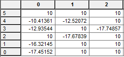
The encoding keys for this file will be

xkey = [0,0,1,0,2,0,1];

ykey = [0,1,2,3,3,4,4];

zkey = [0,0,0,0,0,0,0];

The encoding key array lengths match the number of data values being stored in the file.

If the data is only 2D, then the z key array should contain all zeros. If the data is only 1D, then the y and z key arrays should contain all zeros.

When writing and reading dynamic data items of a compressed file, compression and decompression is handled automatically on the fly, i.e. the user must provide the full 3D array when writing, and is given the full 3D array when reading.

Compression currently works under the following conditions:

• All the dynamic items in the file must have the same spatial axis.

• All the dynamic items must store its data as floats.

Compression and decompression of static items is not supported on DFS file level. Some file types still store only the compressed data, but then defines a dummy 1D spatial axis having the size of the compressed data. Manual compression and decompression by the user is required when writing and reading such static item data.

Statistics Stored in the DFS File

When writing item data to a DFS file, the DFS keeps track of some statistical properties for each item. There are two level of statistics for each item: Global and local.

The global level is the default level. It stores for each item the minimum, the maximum and the number of delete values over all data values, and all time steps.

The local level stores for each data point/grid point/element of an item

• Minimum value.

• Maximum value.

• Mean value.

• Standard deviation.

• Auto correlation

• Number of non-delete values

• Number of delete values

• Number of non-delete value pairs, being the number of times two consecutive time steps both contain non-delete values.

APPENDICES

Modify Times

To ease the use of the temporal axes, when the temporal axes properties are returned by DFS, these can be modified as follows:

• Equidistant time: No modifications take place.

• Non-equidistant time: The start time offset is stored in the file as the time of the first time-step. When reading the file again, the start time offset provides the time of the first time step, while the time of all time steps are subtracted the start time offset such that the first time step returns time 0.

• Equidistant calendar: Start time offset and start date-time is stored in the file as specified. When reading the file again, the start time offset is returned as 0, its value being added to the start date time. If the start time offset contains fractions of seconds, these are lost.

• Non-equidistant calendar: The start time offset is stored in the file as the time of the first time-step. When reading the file again, the start time offset is returned as zero, its value being added to the start date time, and all time step times are subtracted the start time offset such that the first time step returns time 0. If the start time offset (the time of the first time step) contains fractions of seconds, these are lost.

In the .NET API these modifications are by default disabled. Use the DfsParameters class to specify whether times should be modified or not.

In the C-API the modifications are by default enabled. Use the dfsParamModifyTimes method to specify whether times should be modified or not.

Storing Unicode Strings as Items

The assumption in most MIKE products and tools is that strings are stored as ANSI strings (8 bit characters), when naming items etc. in DFS files.

String data in the form of Unicode strings can as such not be stored as data in a dynamic or static item.

A standard string in .NET is a Unicode string and consists of 16 bit characters, and that needs to be converted into a series of bytes (8 bit).

You can store strings in ANSI format by converting them to/from a byte string using the default ANSI encoder. The following two lines of C# code show how to encode and decode ANSI strings into bytes:

byte[] ansiBytes = System.Text.Encoding.Default.GetBytes(‘MyString’);
string mystring  = System.Text.Encoding.Default.GetString(ansiBytes);

The ANSI format depends on the computer at hand; you cannot transfer all characters from a Danish computer to a French computer. That is a general problem for all strings stored in the DFS files, as also for e.g., the item names and file title. Hence special characters as the Danish æ, ø and å may not show up correctly on non-Danish computers.

When storing a string as the data of a static (or dynamic) item, you can also convert the string to UTF-8, which can hold all types of characters that can be stored in a Unicode (C#) string, as bytes. That will make sure that you get the very same string back, that you actually wrote, independent of the computer that read/writes the data.

byte[] unibytes = System.Text.Encoding.UTF8.GetBytes(‘MyString’);
string mystring = System.Text.Encoding.UTF8.GetString(unibytes);

Special characters in such a string will usually not show up correctly in MIKE products and tools.

Description of the Item Value Types

The value type specifies specify how each data value of an item is to be interpreted in time.

• Instantaneous: The values represent the item at the exact times specified. For example, data from an instant measuring devices, as e.g. the wind velocity in [m/s]. Linear variation between the time steps is usually assumed, i.e. to get values in between time steps, linear interpolation can be used.

• Accumulated: The values represent successive accumulation of the item over time, from the start time of the file to the current time. For example, the rainfall accumulated over a year in [mm], and recorded every day. Linear variation between the time steps is usually assumed, i.e. to get values in between time steps, linear interpolation can be used.

• Step Accumulated: The values represent accumulation of the item over one time step, from the previous time step time to the current time step. For example, rainfall measured for a year, recording for every day the amount of rain in [mm] falling that day.

• Mean Step Backward: The values represent the item from the previous time step to the current time step. For example, the average rain rate between the last and the current time step. Also called “mean step accumulated”.

• Mean Step Forward: The values represent the item from the current time step to the next time step. Also called “reverse mean step accumulated”.

The step accumulated is often used in the following context. Say that we start measuring rainfall at 10:00:00. At 11:00:00 we take the measuring device, register the amount of rain it has collected, say it has the value of 10, and empties the device. At 12:00:00 the same process takes place, say with the value of 15, and so on every hour. In a time series we will have the value 10 at time step 11:00:00 and the value 15 at time step 12:00:00 and so on. Values represent the accumulation of the item over a time span covering from the previous time step to the current time step.

The accumulated, step accumulated, and mean step forward and backward value types can represent the exact same data. The Instantaneous value type cannot be directly converted forth and back between the other value types.

Table F. 1 shows how to represent the same rain time series with the 4 different equivalent value types. Note that they do not have the same EUM type and unit.

You convert data from step accumulated values to mean step backward values by dividing the step accumulated value with the time for the time step. Example, from 18:10:00 to 18:12:00 there was 0.36 mm = 360 $\mu m$ of rain within 120 seconds, giving 3 $\mu m/s$ in that period.

The forward and backward step values differ by being switched one place in the table.

Table F. 1 Values for a rain measurement time series for different value types, representing the exact same rain

Time	Accumulated	Step accumulated	Mean step backward	Mean step forward
	[$mm$]	[$mm$]	[$\mu m/s$]	[$\mu m/s$]
18:00:00	0	0	0	0
18:10:00	0	0	0	3
18:12:00	0.36	0.36	3	7
18:15:00	1.62	1.26	7	12
18:16:00	2.34	0.72	12	14
18:20:00	5.70	3.36	14	42
18:22:00	10.74	5.04	42	10
18:24:00	11.94	1.20	10	20
18:27:00	15.54	3.60	20	18
18:28:00	16.62	1.08	18	14
18:29:00	17.46	0.84	14	10
18:32:00	19.26	1.80	10	4
18:34:00	19.74	0.48	4	5
18:40:00	21.54	1.80	5	1
18:47:00	21.96	0.42	1	0
19:00:00	21.96	0	0	0

A graphical interpretation of the different value types is shown in Figure F. 1 - Figure F. 5.

The instantaneous version has the same values as the forward step from Table F.1.

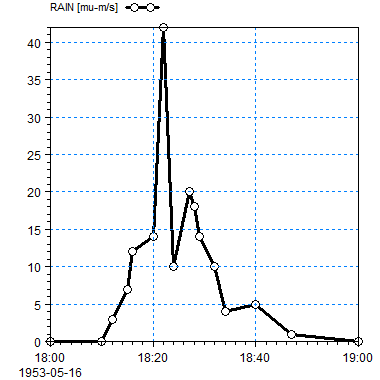
Figure F. 1 Instantaneous value type time series: Points are connected by lines.

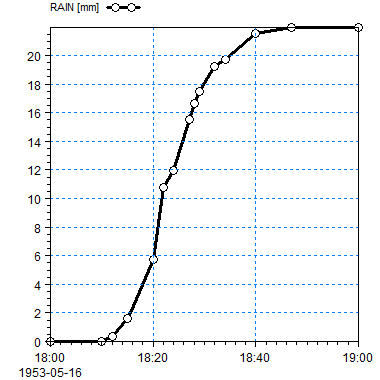
Figure F. 2 Accumulated value type: An Accumulated time series shall always be increasing

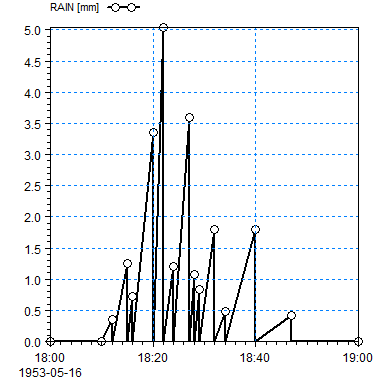
Figure F. 3 Step accumulated value type in a time series: A line is drawn from the x-axis at the previous time step to the data point

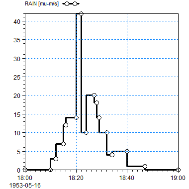
Figure F. 4 Mean step backward value type for a time series: A line is drawn from the previous time step to the current time step with the value at current time step

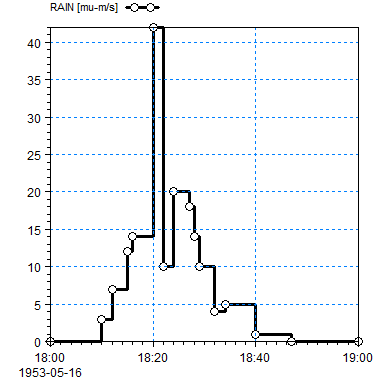
Figure F. 5 Mean step forward value type for a time series: A line is drawn from the current time step to the next time step with the value at the current time step

DFS Data Type Tags Currently Used

Data type tag	Data description	DFS file type	Product suite name
0	Generic data for general use	dfs0+1+2	MIKE Zero
-1	MIKE 21 HD output (H only)	dfs2	MIKE 21
1	M21TRN output	dfs1+2	MIKE 21
1	MIKE 21 HD simulation output (H,P,Q)	dfs1+2	MIKE 21
2	M21TRA output	dfs1+2	MIKE 21
2	MIKE 21 AD,EU,ME,MT,WQ hot start data	dfs1+2	MIKE 21
2	MIKE 21 AD,EU,ME,MT,WQ simulation output	dfs1+2	MIKE 21
3	MIKE 3 HD, AD, EU, ME, MT, WQ simulation output	dfs0+1+2+3	MIKE 3
4	MIKE 21 ST output	dfs2	MIKE 21
11	MIKE 21 HD hot start data	dfs2	MIKE 21
31	MIKE 3 ACM hot start data	dfs3	MIKE 3
32	MIKE 3 ACM input data (HD) for a AD standalone simulation	dfs3	MIKE 3
33	MIKE 3 HD, AD, EU, ME, MT, WQ simulation output (vertical plane)	dfs2	MIKE 3
34	MIKE 3 HD structure output	dfs0	MIKE 3
35	MIKE 3 HS hot start data	dfs3	MIKE 3
36	MIKE 3 HS input data (HD) for a AD standalone simulation	dfs3	MIKE 3
51	M21NPA output hot data	dfs0	MIKE 21
51	M21PA output hot data	dfs0	MIKE 21
61	M21SA output hot data	dfs0	MIKE 21
71	M21RMS output	dfs2	MIKE 21
101	Cross-shore profile	dfs1	LITPACK
102	Timeseries wave climate	dfs0	LITPACK
103	Event duration wave climate	dfs2	LITPACK
104	Time series for LITSTP	dfs0	LITPACK
105	Coastline alignment	dfs1	LITPACK
106	Cross-section of trench	dfs1	LITPACK
107	Wave events for LITPROF	dfs0	LITPACK
108	Source file for LITLINE	dfs0	LITPACK
109	Wave events for LITTREN	dfs0	LITPACK
111	LITDRIFT output (Littoral current)	dfs1	LITPACK
112	LITDRIFT output (Littoral drift)	dfs1	LITPACK
113	LITDRIFT output (Littoral budget)	dfs0+1	LITPACK
114	LITDRIFT output (Budget rose))	dfs0	LITPACK
116	LITSTP output (single event)	dfs0	LITPACK
117	LITSTP output (single event, extended output)	dfs0+1	LITPACK
118	LITSTP output (time series events)	dfs0+1	LITPACK
120	LITPROF output	dfs1	LITPACK
121	LITLINE output	dfs1	LITPACK
122	LITTREN output	dfs1	LITPACK
217	CONTROL SIGNAL FILE	dfs1	Wave Syntheziser
217	WS Wave generated control signals (WS_WG_DATA)	dfs1	Wave Syntheziser
218	WS_DAQ_DATA	unknown	Wave Syntheziser
219	WS data acquired by WS controller component (WS_DAQ_DATA_RECALIBRATED)	unknown	Wave Syntheziser
220	WS_AWACS_DATA	unknown	Wave Syntheziser
221	WS_AWACS_REFLECTION_DATA	unknown	Wave Syntheziser
222	WS_SPECTRAL_DATA	unknown	Wave Syntheziser
223	WS_CROSSING_DATA	unknown	Wave Syntheziser
224	WS_REFLECTION_DATA	unknown	Wave Syntheziser
225	WS_FILTERING_DATA	unknown	Wave Syntheziser
230	WS_DIRECTIONAL_DATA	unknown	Wave Syntheziser
240	WS_MATLAB_DATA	unknown	Wave Syntheziser
250	WS_NORTEK_ADV_DATA	unknown	Wave Syntheziser
800	Pier data for MIKE 21 HD	dfs1	MIKE 21
901	ADCP current data for ADCPLT	dfs1	MIKE Zero
930	Radiation stresses	dfs2	MIKE 21
2000	Flow Model FM, Finite Element data file + mesh data	dfsu	MIKE FM
2001	Flow Model FM, Finite Volume data file	dfsu	MIKE FM
2002	Spectral Wave Model FM, Finite Element data file	dfsu	MIKE FM
2003	Spectra Wave Model FM, Finite Volume data file	dfsu	MIKE FM
3000	Layer data from GEO Model	dfs2	MIKE GEOModel
10001	Output from Grd2Mike tool	dfs2	MIKE Zero
10001	MIKE SHE general 2D result file (all model cells)	dfs2	MIKE SHE
10002	MIKE SHE 2D UZ result file (UZ cells), static items containing mapping from UZ cell to model cell	dfs2	MIKE SHE
10003	MIKE SHE 3D UZ result file (UZ nodes, UZ cells), static items containing mapping from UZ cell to model cell	dfs3	MIKE SHE
10004	MIKE SHE 3D SZ Flow result file (all model cells X SZ layers), static items containing hydro-geologic properties	dfs3	MIKE SHE
10005	MIKE SHE 3D SZ "non-Flow" result file (all model cells X SZ layers), static items containing hydro-geologic properties	dfs3	MIKE SHE
10006	MIKE SHE 3D SZ "others" result file (all model cells X SZ layers), without hydro-properties as static items	dfs3	MIKE SHE